TorchRL 强化学习 (PPO) 教程 ¶

译者：片刻小哥哥

项目地址：https://pytorch.apachecn.org/2.0/tutorials/intermediate/reinforcement_ppo

原始地址：https://pytorch.org/tutorials/intermediate/reinforcement_ppo.html

作者 : 文森特·莫恩斯

本教程演示如何使用 PyTorch 和 torchrl 训练参数策略 网络以解决 OpenAI-Gym/Farama-Gymnasium 控制库 .

倒立摆 ¶

主要经验教训：

• 如何在 TorchRL 中创建一个环境，转换其输出，并从该环境中收集数据；
• 如何使用 TensorDict 让你的类相互对话 ;

• 构建训练的基础知识使用 TorchRL 循环:

  • 如何计算策略梯度方法的优势信号；
  • 如何使用概率神经网络创建随机策略；
  • 如何创建动态重播缓冲区并从中进行不重复的采样。

我们将介绍 TorchRL 的六个关键组成部分：

• 环境
• 变换
• 模型(策略和价值函数)
• 损失模块\ n* 数据收集器
• 重播缓冲区

如果您在 Google Colab 中运行此程序，请确保安装以下依赖项：

!pip3 install torchrl
!pip3 install gym[mujoco]
!pip3 install tqdm

邻近策略优化 (PPO) 是一种策略梯度算法， 正在收集一批数据并直接使用它来训练策略，以在给定一些邻近性约束的情况下最大化 预期回报。您可以将其视为基础策略优化算法的复杂版本 REINFORCE。有关详细信息，请参阅 近端策略优化算法 论文。

PPO 通常被认为是一种快速有效的在线同策略强化算法方法。 TorchRL 提供了一个损失模块， 为您完成所有工作，以便您可以依赖此实现并专注于解决 问题，而不是每次想要训练策略时都重新发明轮子。

为了完整起见，这里简要概述了损失的计算内容，尽管 这是由我们的 ClipPPOLoss module—该算法的工作原理如下： 1.我们将通过在环境中执行给定步骤数的策略来采样一批数据。 2.然后，我们将使用增强损失的剪裁版本对该批次的随机子样本执行给定数量的优化步骤。 3.剪裁会给我们的损失带来悲观的界限：与较高的收益估计相比，较低的收益估计 会更受欢迎。 损失的精确公式为：

[L(s,a,\theta_k,\theta) = \min\left( \frac{\pi_{\theta}(a| s)}{\pi_{\theta_k}(a|s)} A^{\pi_{\theta_k}}(s,a), \ ;\; g(\epsilon, A^{\pi_{\theta_k}}(s,a)) \right),]

\该损失有两个组成部分：在最小运算符的第一部分中， 我们只是计算 REINFORCE 损失的重要性加权版本(例如， 我们已针对当前策略的事实进行了纠正的 REINFORCE 损失 配置滞后于用于数据收集的配置。 最小运算符的第二部分是类似的损失，当比率超过或低于给定的一对阈值时，我们会剪裁 比率。

这种损失确保了无论优势是正面还是负面， 不鼓励那些与之前的配置产生重大变化的策略更新。

本教程的结构如下：

1. 首先，我们将定义一组用于训练的超参数。 2.接下来，我们将专注于使用 TorchRL’s 包装器和转换来创建我们的环境或模拟器。 3.接下来，我们将设计策略网络和价值模型，这对于损失函数来说是不可或缺的。这些模块将用于配置我们的损失模块。 4.接下来，我们将创建重播缓冲区和数据加载器。 5.最后，我们将运行训练循环并分析结果。

在整个教程中，我们’ 将使用 tensordict 库。 TensorDict 是 TorchRL 的通用语言：它帮助我们抽象 模块读取和写入的内容不太关心具体的数据 描述，而更多地关心算法本身。

from collections import defaultdict

import matplotlib.pyplot as plt
import torch
from tensordict.nn import TensorDictModule
from tensordict.nn.distributions import NormalParamExtractor
from torch import nn
from torchrl.collectors import SyncDataCollector
from torchrl.data.replay_buffers import ReplayBuffer
from torchrl.data.replay_buffers.samplers import SamplerWithoutReplacement
from torchrl.data.replay_buffers.storages import LazyTensorStorage
from torchrl.envs import (Compose, DoubleToFloat, ObservationNorm, StepCounter,
                          TransformedEnv)
from torchrl.envs.libs.gym import GymEnv
from torchrl.envs.utils import check_env_specs, set_exploration_mode
from torchrl.modules import ProbabilisticActor, TanhNormal, ValueOperator
from torchrl.objectives import ClipPPOLoss
from torchrl.objectives.value import GAE
from tqdm import tqdm

定义超参数 ¶

我们为算法设置超参数。根据 可用的资源，可以选择在 GPU 或另一 设备上执行策略。 frame_skip 将控制单个操作 执行的帧数。计算帧数的其余参数 必须针对此值进行更正(因为一个环境步骤 实际上会返回 frame_skip 帧)。

device = "cpu" if not torch.cuda.is_available() else "cuda:0"
num_cells = 256  # number of cells in each layer i.e. output dim.
lr = 3e-4
max_grad_norm = 1.0

数据收集参数 ¶

收集数据时，我们可以通过定义 frames_per_batch 参数来选择每个批次的大小。我们还将定义我们允许自己使用的 帧数(例如与模拟器的交互次数)。一般来说，RL 算法的目标是在环境交互方面尽可能快地学习解决任务： total_frames 越低越好。 我们还定义了 n frame_skip ：在某些情况下，在轨迹过程中 多次重复相同的操作可能是有益的，因为 它使行为更加一致且不那么不稳定。但是，“ 跳过” 过多的帧会降低参与者对观察变化的反应性，从而阻碍训练。

使用 frame_skip 时，最好根据我们分组的帧数 更正其他帧计数。如果我们配置 X 帧的总数进行训练，但 使用 Y 的 frame_skip ，我们实际上将收集

XY 帧总数，这超出了我们预定义的预算。

frame_skip = 1
frames_per_batch = 1000 // frame_skip
# For a complete training, bring the number of frames up to 1M
total_frames = 50_000 // frame_skip

PPO 参数 ¶

在每次数据收集(或批量收集)时，我们将在一定数量的 epochs 上运行优化，每次都会消耗我们在嵌套训练循环中 刚刚获取的整个数据。这里， sub_batch_size 与上面的 frames_per_batch 不同：回想一下，我们正在使用 “batch data” 来自我们的收集器，其大小由 frames_per_batch 定义，并且 我们将在内部训练循环期间进一步拆分为更小的子批次。 这些子批次的大小由 sub_batch_size 控制。

sub_batch_size = 64  # cardinality of the sub-samples gathered from the current data in the inner loop
num_epochs = 10  # optimization steps per batch of data collected
clip_epsilon = (
    0.2  # clip value for PPO loss: see the equation in the intro for more context.
)
gamma = 0.99
lmbda = 0.95
entropy_eps = 1e-4

定义环境 ¶

在强化学习中， 环境 通常是我们指代模拟器或控制系统的方式。各种库提供了用于强化学习的模拟环境，包括 Gymnasium(以前称为 OpenAI Gym)、DeepMind Control Suite 等。 作为通用库，TorchRL’s 的目标是提供一个可互换的接口 大型 RL 模拟器面板，让您可以轻松地在一个环境与另一个环境之间切换 。例如，只需几个字符即可创建一个包装式健身房环境：

base_env = GymEnv("InvertedDoublePendulum-v4", device=device, frame_skip=frame_skip)

这段代码中有几件事需要注意：首先，我们通过调用 GymEnv 包装器创建 环境。如果传递了额外的关键字参数，它们将被传送到 gym.make 方法，从而覆盖 最常见的环境构建命令。 或者，也可以使用 `直接创建一个gym环境。 gym.make(env_name,

**kwargs)` 并将其包装在

GymWrapper

类中。

还有 device 参数：对于gym，这仅控制存储输入操作和观察到的状态的设备，但执行将始终在CPU 上完成。原因很简单，除非另有说明，否则gym不支持设备上执行 。对于其他库，我们可以控制执行设备，并尽可能在存储和执行后端方面保持一致。

转换 ¶

我们将在我们的环境中附加一些转换，以 为策略准备数据。在 Gym 中，这通常是通过包装器来实现的。 TorchRL 采用了一种不同的方法，通过使用变换，与其他 pytorch 域库更相似。 要将变换添加到环境中，只需将其包装在 TransformedEnv 实例并将变换序列附加到它。转换后的环境将继承 包装环境的设备和元数据，并根据其包含的 转换序列对它们进行转换。

标准化 ¶

第一个编码是归一化变换。 根据经验，最好有松散匹配单位高斯分布的数据： 为了获得此结果，我们将 在环境中运行一定数量的随机步骤并计算 这些观察结果的汇总统计数据。

我们’ll 附加两个其他转换： DoubleToFloat 转换会将双精度数 转换为单精度数字，以供策略读取。

StepCounter 转换将用于计算 环境终止之前的步数。我们将使用此衡量标准作为 性能的补充衡量标准。

正如我们稍后将看到的，许多 TorchRL’s 类依赖 TensorDict 进行通信。您可以将其视为具有一些额外 tensor功能的 Python 字典。实际上，这意味着我们将要使用的许多模块 需要被告知要读取什么键( in_keys )以及要写入 ( out_keys ) 在他们将收到的 tensordict 中。通常，如果省略 out_keys ，则假定 in_keys 条目将就地更新。对于我们的变换，我们感兴趣的唯一条目被称为 “观察” ，并且我们的变换层将被告知修改此 条目并且仅修改此条目：

env = TransformedEnv(
    base_env,
    Compose(
        # normalize observations
        ObservationNorm(in_keys=["observation"]),
        DoubleToFloat(in_keys=["observation"]),
        StepCounter(),
    ),
)

正如您可能已经注意到的，我们创建了一个归一化层，但我们没有 设置其归一化参数。为此， ObservationNorm 可以 自动收集我们环境的摘要统计信息:

env.transform[0].init_stats(num_iter=1000, reduce_dim=0, cat_dim=0)

ObservationNorm 变换现已填充 用于标准化数据的位置和比例。

让我们对摘要统计数据的形状进行一些健全性检查：

print("normalization constant shape:", env.transform[0].loc.shape)

normalization constant shape: torch.Size([11])

环境不仅由其模拟器和转换来定义， 还由一系列元数据定义，这些元数据描述了 执行过程中的预期情况。 出于效率目的，TorchRL 在环境方面非常严格 规范，但您可以轻松检查您的环境规范是否足够。 在我们的示例中，继承自它的 GymWrapper 和 GymEnv 已经负责设置正确的规范您的环境，因此 您不必关心这个。

尽管如此，让 ’s 通过查看其规格来查看使用我们转换后的 环境的具体示例。 需要查看三个规格： observation_spec 定义了什么 在环境中执行操作时预期的 reward_spec 指示奖励域，最后是 input_spec (其中包含 action_spec ) 并代表 环境执行单个步骤所需的一切。

print("observation_spec:", env.observation_spec)
print("reward_spec:", env.reward_spec)
print("input_spec:", env.input_spec)
print("action_spec (as defined by input_spec):", env.action_spec)

observation_spec: CompositeSpec(
    observation: UnboundedContinuousTensorSpec(
        shape=torch.Size([11]),
        space=None,
        device=cuda:0,
        dtype=torch.float32,
        domain=continuous),
    step_count: BoundedTensorSpec(
        shape=torch.Size([1]),
        space=ContinuousBox(
            low=Tensor(shape=torch.Size([1]), device=cuda:0, dtype=torch.int64, contiguous=True),
            high=Tensor(shape=torch.Size([1]), device=cuda:0, dtype=torch.int64, contiguous=True)),
        device=cuda:0,
        dtype=torch.int64,
        domain=continuous), device=cuda:0, shape=torch.Size([]))
reward_spec: UnboundedContinuousTensorSpec(
    shape=torch.Size([1]),
    space=ContinuousBox(
        low=Tensor(shape=torch.Size([1]), device=cuda:0, dtype=torch.float32, contiguous=True),
        high=Tensor(shape=torch.Size([1]), device=cuda:0, dtype=torch.float32, contiguous=True)),
    device=cuda:0,
    dtype=torch.float32,
    domain=continuous)
input_spec: CompositeSpec(
    full_state_spec: CompositeSpec(
        step_count: BoundedTensorSpec(
            shape=torch.Size([1]),
            space=ContinuousBox(
                low=Tensor(shape=torch.Size([1]), device=cuda:0, dtype=torch.int64, contiguous=True),
                high=Tensor(shape=torch.Size([1]), device=cuda:0, dtype=torch.int64, contiguous=True)),
            device=cuda:0,
            dtype=torch.int64,
            domain=continuous), device=cuda:0, shape=torch.Size([])),
    full_action_spec: CompositeSpec(
        action: BoundedTensorSpec(
            shape=torch.Size([1]),
            space=ContinuousBox(
                low=Tensor(shape=torch.Size([1]), device=cuda:0, dtype=torch.float32, contiguous=True),
                high=Tensor(shape=torch.Size([1]), device=cuda:0, dtype=torch.float32, contiguous=True)),
            device=cuda:0,
            dtype=torch.float32,
            domain=continuous), device=cuda:0, shape=torch.Size([])), device=cuda:0, shape=torch.Size([]))
action_spec (as defined by input_spec): BoundedTensorSpec(
    shape=torch.Size([1]),
    space=ContinuousBox(
        low=Tensor(shape=torch.Size([1]), device=cuda:0, dtype=torch.float32, contiguous=True),
        high=Tensor(shape=torch.Size([1]), device=cuda:0, dtype=torch.float32, contiguous=True)),
    device=cuda:0,
    dtype=torch.float32,
    domain=continuous)

check_env_specs() 函数运行一次小型部署，并将其输出与环境规范进行比较。 如果没有出现错误，我们可以确信规范已正确定义：

check_env_specs(env)

check_env_specs succeeded!

为了好玩，让’s 看看简单的随机推出是什么样子的。您可以 调用

env.rollout(n_steps)

并大致了解环境输入 和输出的样子。操作将自动从操作规范 域中提取，因此您’无需关心设计随机采样器。

通常，在每一步，强化学习环境都会接收一个动作作为输入，并输出一个观察结果、一个奖励和一个完成状态。观测值可能是复合的，这意味着它可能由多个tensor组成。对于 TorchRL 来说这不是问题，因为整个观察集会自动打包在输出中TensorDict 中。在给定的步骤数上执行 rollout(例如，一系列环境步骤和随机操作生成)后，我们将检索一个形状与轨迹长度匹配的“TensorDict”实例：

rollout = env.rollout(3)
print("rollout of three steps:", rollout)
print("Shape of the rollout TensorDict:", rollout.batch_size)

rollout of three steps: TensorDict(
    fields={
        action: Tensor(shape=torch.Size([3, 1]), device=cuda:0, dtype=torch.float32, is_shared=True),
        done: Tensor(shape=torch.Size([3, 1]), device=cuda:0, dtype=torch.bool, is_shared=True),
        next: TensorDict(
            fields={
                done: Tensor(shape=torch.Size([3, 1]), device=cuda:0, dtype=torch.bool, is_shared=True),
                observation: Tensor(shape=torch.Size([3, 11]), device=cuda:0, dtype=torch.float32, is_shared=True),
                reward: Tensor(shape=torch.Size([3, 1]), device=cuda:0, dtype=torch.float32, is_shared=True),
                step_count: Tensor(shape=torch.Size([3, 1]), device=cuda:0, dtype=torch.int64, is_shared=True),
                terminated: Tensor(shape=torch.Size([3, 1]), device=cuda:0, dtype=torch.bool, is_shared=True),
                truncated: Tensor(shape=torch.Size([3, 1]), device=cuda:0, dtype=torch.bool, is_shared=True)},
            batch_size=torch.Size([3]),
            device=cuda:0,
            is_shared=True),
        observation: Tensor(shape=torch.Size([3, 11]), device=cuda:0, dtype=torch.float32, is_shared=True),
        step_count: Tensor(shape=torch.Size([3, 1]), device=cuda:0, dtype=torch.int64, is_shared=True),
        terminated: Tensor(shape=torch.Size([3, 1]), device=cuda:0, dtype=torch.bool, is_shared=True),
        truncated: Tensor(shape=torch.Size([3, 1]), device=cuda:0, dtype=torch.bool, is_shared=True)},
    batch_size=torch.Size([3]),
    device=cuda:0,
    is_shared=True)
Shape of the rollout TensorDict: torch.Size([3])

我们的推出数据的形状为 torch.Size([3]) ，它与我们运行它的步骤数 相匹配。 "next" 条目指向当前步骤之后的数据。 在大多数情况下， "next" 时刻的数据

t

与数据匹配at t+1 ，但如果我们使用一些特定的转换(例如，多步)，情况可能并非如此。

策略 ¶

PPO 利用随机策略来处理探索。这意味着我们的神经网络必须输出分布的参数，而不是与所采取的操作相对应的单个值。

由于数据是连续的，我们使用 Tanh 正态分布来尊重 动作空间边界。 TorchRL 提供了这样的分布， 我们唯一需要关心的是构建一个神经网络， 输出正确数量的参数供策略使用(位置或平均值， 和比例)：

[f_{\theta}(\text{观察}) = \mu_{\theta}(\text{观察}), \sigma^{+} _{\theta}(\text{observation})]

这里提出的唯一额外困难是将我们的输出分成两部分，并将第二部分映射到严格的正空间。

我们分三步设计策略：

1. 定义神经网络 D_obs -> `2

*

D_action。事实上，我们的loc(mu) 和scale(sigma) 都有维度D_action。 2.附加NormalParamExtractor以提取位置和比例(例如，将输入分成两等份并对比例参数应用正变换)。 3.创建一个概率TensorDictModule` 可以生成此分布并从中采样。

actor_net = nn.Sequential(
    nn.LazyLinear(num_cells, device=device),
    nn.Tanh(),
    nn.LazyLinear(num_cells, device=device),
    nn.Tanh(),
    nn.LazyLinear(num_cells, device=device),
    nn.Tanh(),
    nn.LazyLinear(2 * env.action_spec.shape[-1], device=device),
    NormalParamExtractor(),
)

/opt/conda/envs/py_3.10/lib/python3.10/site-packages/torch/nn/modules/lazy.py:180: UserWarning:

Lazy modules are a new feature under heavy development so changes to the API or functionality can happen at any moment.

为了使策略能够通过 tensordict 数据载体“talk” 与环境进行对话，我们将 nn.Module 包装在一个 TensorDictModule .该类将简单地准备好它所提供的 in_keys 并在注册的 out_keys 处写入 输出。

policy_module = TensorDictModule(
    actor_net, in_keys=["observation"], out_keys=["loc", "scale"]
)

我们现在需要根据正态分布的位置和规模构建一个分布。为此，我们指示 ProbabilisticActor 构建一个 TanhNormal 超出位置和比例 参数。我们还提供了从环境规范中收集的 分布的最小值和最大值。

in_keys 的名称(以及上面的 TensorDictModule 的 out_keys 的名称)不能设置为任何值一可能 喜欢，如 TanhNormal 分发构造函数将需要 loc 和 scale 关键字参数。话虽如此， ProbabilisticActor 还接受 `Dict[str,

str]键入in_keys其中键值对表示 什么in_key` 字符串应该用于要使用的每个关键字参数。

policy_module = ProbabilisticActor(
    module=policy_module,
    spec=env.action_spec,
    in_keys=["loc", "scale"],
    distribution_class=TanhNormal,
    distribution_kwargs={
        "min": env.action_spec.space.minimum,
        "max": env.action_spec.space.maximum,
    },
    return_log_prob=True,
    # we'll need the log-prob for the numerator of the importance weights
)

价值网络 ¶

价值网络是 PPO 算法的重要组成部分，尽管它 不能在推理时使用’。该模块将读取观察结果并 返回以下轨迹的折扣回报的估计。 这使我们能够通过依赖在训练期间动态学习的一些效用估计 来摊销学习。我们的价值网络与策略共享 相同的结构，但为了简单起见，我们为其分配了自己的 参数集。

value_net = nn.Sequential(
    nn.LazyLinear(num_cells, device=device),
    nn.Tanh(),
    nn.LazyLinear(num_cells, device=device),
    nn.Tanh(),
    nn.LazyLinear(num_cells, device=device),
    nn.Tanh(),
    nn.LazyLinear(1, device=device),
)

value_module = ValueOperator(
    module=value_net,
    in_keys=["observation"],
)

/opt/conda/envs/py_3.10/lib/python3.10/site-packages/torch/nn/modules/lazy.py:180: UserWarning:

Lazy modules are a new feature under heavy development so changes to the API or functionality can happen at any moment.

让’s 尝试我们的策略和值模块。正如我们之前所说，使用 TensorDictModule 可以直接读取 环境的输出来运行这些模块，因为它们知道要读取 哪些信息以及将其写入何处：

print("Running policy:", policy_module(env.reset()))
print("Running value:", value_module(env.reset()))

Running policy: TensorDict(
    fields={
        action: Tensor(shape=torch.Size([1]), device=cuda:0, dtype=torch.float32, is_shared=True),
        done: Tensor(shape=torch.Size([1]), device=cuda:0, dtype=torch.bool, is_shared=True),
        loc: Tensor(shape=torch.Size([1]), device=cuda:0, dtype=torch.float32, is_shared=True),
        observation: Tensor(shape=torch.Size([11]), device=cuda:0, dtype=torch.float32, is_shared=True),
        sample_log_prob: Tensor(shape=torch.Size([]), device=cuda:0, dtype=torch.float32, is_shared=True),
        scale: Tensor(shape=torch.Size([1]), device=cuda:0, dtype=torch.float32, is_shared=True),
        step_count: Tensor(shape=torch.Size([1]), device=cuda:0, dtype=torch.int64, is_shared=True),
        terminated: Tensor(shape=torch.Size([1]), device=cuda:0, dtype=torch.bool, is_shared=True),
        truncated: Tensor(shape=torch.Size([1]), device=cuda:0, dtype=torch.bool, is_shared=True)},
    batch_size=torch.Size([]),
    device=cuda:0,
    is_shared=True)
Running value: TensorDict(
    fields={
        done: Tensor(shape=torch.Size([1]), device=cuda:0, dtype=torch.bool, is_shared=True),
        observation: Tensor(shape=torch.Size([11]), device=cuda:0, dtype=torch.float32, is_shared=True),
        state_value: Tensor(shape=torch.Size([1]), device=cuda:0, dtype=torch.float32, is_shared=True),
        step_count: Tensor(shape=torch.Size([1]), device=cuda:0, dtype=torch.int64, is_shared=True),
        terminated: Tensor(shape=torch.Size([1]), device=cuda:0, dtype=torch.bool, is_shared=True),
        truncated: Tensor(shape=torch.Size([1]), device=cuda:0, dtype=torch.bool, is_shared=True)},
    batch_size=torch.Size([]),
    device=cuda:0,
    is_shared=True)

数据收集器 ¶

TorchRL 提供了一组 DataCollector 类 。 简而言之，这些类执行三个操作：重置环境、 计算操作根据最新的观察结果，在环境中执行一个步骤， 并重复最后两个步骤，直到环境发出停止信号(或达到 完成状态)。

它们允许您控制每次迭代时收集多少帧 (通过 frames_per_batch 参数)， 何时重置环境(通过 max\ \_frames_per_traj 参数)、 应执行哪个 设备 策略等。它们还 设计用于在批处理和多处理环境中高效工作。

最简单的数据收集器是 SyncDataCollector : it 是一个迭代器，可用于获取给定长度的批量数据，并且 一旦达到总帧数 ( total\ _frames ) 已 收集。 其他数据收集器 ( MultiSyncDataCollector 和 MultiaSyncDataCollector ) 将在一组多进程工作线程上以同步和异步方式执行 相同的操作。

对于之前的策略和环境，数据收集器将返回 TensorDict 个实例，其元素总数将 匹配

frames_per_batch 。使用 TensorDict 将数据传递到 训练循环允许您编写 数据加载管道， 这些管道 100% 不关心推出内容的实际特殊性。

collector = SyncDataCollector(
    env,
    policy_module,
    frames_per_batch=frames_per_batch,
    total_frames=total_frames,
    split_trajs=False,
    device=device,
)

重播缓冲区 ¶

重播缓冲区是离策略 RL 算法的常见构建部分。 在同策略上下文中，每次收集一批数据时都会重新填充重播缓冲区， 并且其数据会被重复消耗一定数量的 纪元。

TorchRL’s 重播缓冲区是使用通用容器构建的 ReplayBuffer 它将缓冲区的组件 作为参数：存储、写入器、采样器以及可能的一些转换。 仅存储(指示重播)缓冲区容量)是强制性的。 我们还指定一个不重复的采样器，以避免在一个 epoch 中对同一项目进行多次采样。 对 PPO 使用重播缓冲区不是强制性的，我们可以简单地 从收集到的子批次中进行采样批处理，但使用这些类 使我们可以轻松地以可重现的方式构建内部训练循环。

replay_buffer = ReplayBuffer(
    storage=LazyTensorStorage(frames_per_batch),
    sampler=SamplerWithoutReplacement(),
)

损失函数 ¶

为了方便起见，可以使用 ClipPPOLoss 直接从 TorchRL 导入 PPO 损失“(在 torchrl vmain (0.2.1 )) 中”) 类。这是利用 PPO 的最简单方法： 它隐藏了 PPO 的数学运算以及随之而来的控制流。

PPO 需要计算一些“advantage 估计”。简而言之，优势 是一个在处理偏差/方差权衡时反映对返回值的期望的值。 要计算优势，只需 (1) 构建优势模块， 利用我们的值运算符，并且 (2) 在每个 epoch之前传递每批数据。 GAE 模块将使用新的 "advantage" 和 "值更新输入tensordict_target" 个条目。

"value_target" 是一个无梯度tensor，表示价值网络应使用输入观测表示的 经验值。 这两者都将由 ClipPPOLoss

退回保单和价值损失。

advantage_module = GAE(
    gamma=gamma, lmbda=lmbda, value_network=value_module, average_gae=True
)

loss_module = ClipPPOLoss(
    actor=policy_module,
    critic=value_module,
    advantage_key="advantage",
    clip_epsilon=clip_epsilon,
    entropy_bonus=bool(entropy_eps),
    entropy_coef=entropy_eps,
    # these keys match by default but we set this for completeness
    value_target_key=advantage_module.value_target_key,
    critic_coef=1.0,
    gamma=0.99,
    loss_critic_type="smooth_l1",
)

optim = torch.optim.Adam(loss_module.parameters(), lr)
scheduler = torch.optim.lr_scheduler.CosineAnnealingLR(
    optim, total_frames // frames_per_batch, 0.0
)

训练循环 ¶

现在我们已经拥有了对训练循环进行编码所需的所有部分。 步骤包括：

• 收集数据

  • 计算优势

    • 循环收集以计算损失值
    • 反向传播
    • 优化
    • 重复
      • 重复
    • 重复

logs = defaultdict(list)
pbar = tqdm(total=total_frames * frame_skip)
eval_str = ""

# We iterate over the collector until it reaches the total number of frames it was
# designed to collect:
for i, tensordict_data in enumerate(collector):
    # we now have a batch of data to work with. Let's learn something from it.
    for _ in range(num_epochs):
        # We'll need an "advantage" signal to make PPO work.
        # We re-compute it at each epoch as its value depends on the value
        # network which is updated in the inner loop.
        advantage_module(tensordict_data)
        data_view = tensordict_data.reshape(-1)
        replay_buffer.extend(data_view.cpu())
        for _ in range(frames_per_batch // sub_batch_size):
            subdata = replay_buffer.sample(sub_batch_size)
            loss_vals = loss_module(subdata.to(device))
            loss_value = (
                loss_vals["loss_objective"]
                + loss_vals["loss_critic"]
                + loss_vals["loss_entropy"]
            )

            # Optimization: backward, grad clipping and optimization step
            loss_value.backward()
            # this is not strictly mandatory but it's good practice to keep
            # your gradient norm bounded
            torch.nn.utils.clip_grad_norm_(loss_module.parameters(), max_grad_norm)
            optim.step()
            optim.zero_grad()

    logs["reward"].append(tensordict_data["next", "reward"].mean().item())
    pbar.update(tensordict_data.numel() * frame_skip)
    cum_reward_str = (
        f"average reward={logs['reward'][-1]: 4.4f} (init={logs['reward'][0]: 4.4f})"
    )
    logs["step_count"].append(tensordict_data["step_count"].max().item())
    stepcount_str = f"step count (max): {logs['step_count'][-1]}"
    logs["lr"].append(optim.param_groups[0]["lr"])
    lr_str = f"lr policy: {logs['lr'][-1]: 4.4f}"
    if i % 10 == 0:
        # We evaluate the policy once every 10 batches of data.
        # Evaluation is rather simple: execute the policy without exploration
        # (take the expected value of the action distribution) for a given
        # number of steps (1000, which is our ``env`` horizon).
        # The ``rollout`` method of the ``env`` can take a policy as argument:
        # it will then execute this policy at each step.
        with set_exploration_mode("mean"), torch.no_grad():
            # execute a rollout with the trained policy
            eval_rollout = env.rollout(1000, policy_module)
            logs["eval reward"].append(eval_rollout["next", "reward"].mean().item())
            logs["eval reward (sum)"].append(
                eval_rollout["next", "reward"].sum().item()
            )
            logs["eval step_count"].append(eval_rollout["step_count"].max().item())
            eval_str = (
                f"eval cumulative reward: {logs['eval reward (sum)'][-1]: 4.4f} "
                f"(init: {logs['eval reward (sum)'][0]: 4.4f}), "
                f"eval step-count: {logs['eval step_count'][-1]}"
            )
            del eval_rollout
    pbar.set_description(", ".join([eval_str, cum_reward_str, stepcount_str, lr_str]))

    # We're also using a learning rate scheduler. Like the gradient clipping,
    # this is a nice-to-have but nothing necessary for PPO to work.
    scheduler.step()

  0%|          | 0/50000 [00:00<?, ?it/s]
  2%|2         | 1000/50000 [00:06<05:12, 156.88it/s]
eval cumulative reward:  82.5343 (init:  82.5343), eval step-count: 8, average reward= 9.0890 (init= 9.0890), step count (max): 17, lr policy:  0.0003:   2%|2         | 1000/50000 [00:06<05:12, 156.88it/s]
eval cumulative reward:  82.5343 (init:  82.5343), eval step-count: 8, average reward= 9.0890 (init= 9.0890), step count (max): 17, lr policy:  0.0003:   4%|4         | 2000/50000 [00:12<04:46, 167.61it/s]
eval cumulative reward:  82.5343 (init:  82.5343), eval step-count: 8, average reward= 9.1238 (init= 9.0890), step count (max): 15, lr policy:  0.0003:   4%|4         | 2000/50000 [00:12<04:46, 167.61it/s]
eval cumulative reward:  82.5343 (init:  82.5343), eval step-count: 8, average reward= 9.1238 (init= 9.0890), step count (max): 15, lr policy:  0.0003:   6%|6         | 3000/50000 [00:17<04:34, 171.16it/s]
eval cumulative reward:  82.5343 (init:  82.5343), eval step-count: 8, average reward= 9.1421 (init= 9.0890), step count (max): 15, lr policy:  0.0003:   6%|6         | 3000/50000 [00:17<04:34, 171.16it/s]
eval cumulative reward:  82.5343 (init:  82.5343), eval step-count: 8, average reward= 9.1421 (init= 9.0890), step count (max): 15, lr policy:  0.0003:   8%|8         | 4000/50000 [00:23<04:27, 171.69it/s]
eval cumulative reward:  82.5343 (init:  82.5343), eval step-count: 8, average reward= 9.1779 (init= 9.0890), step count (max): 23, lr policy:  0.0003:   8%|8         | 4000/50000 [00:23<04:27, 171.69it/s]
eval cumulative reward:  82.5343 (init:  82.5343), eval step-count: 8, average reward= 9.1779 (init= 9.0890), step count (max): 23, lr policy:  0.0003:  10%|#         | 5000/50000 [00:29<04:17, 174.74it/s]
eval cumulative reward:  82.5343 (init:  82.5343), eval step-count: 8, average reward= 9.1906 (init= 9.0890), step count (max): 20, lr policy:  0.0003:  10%|#         | 5000/50000 [00:29<04:17, 174.74it/s]
eval cumulative reward:  82.5343 (init:  82.5343), eval step-count: 8, average reward= 9.1906 (init= 9.0890), step count (max): 20, lr policy:  0.0003:  12%|#2        | 6000/50000 [00:34<04:08, 176.79it/s]
eval cumulative reward:  82.5343 (init:  82.5343), eval step-count: 8, average reward= 9.2260 (init= 9.0890), step count (max): 30, lr policy:  0.0003:  12%|#2        | 6000/50000 [00:34<04:08, 176.79it/s]
eval cumulative reward:  82.5343 (init:  82.5343), eval step-count: 8, average reward= 9.2260 (init= 9.0890), step count (max): 30, lr policy:  0.0003:  14%|#4        | 7000/50000 [00:40<04:02, 177.45it/s]
eval cumulative reward:  82.5343 (init:  82.5343), eval step-count: 8, average reward= 9.2230 (init= 9.0890), step count (max): 28, lr policy:  0.0003:  14%|#4        | 7000/50000 [00:40<04:02, 177.45it/s]
eval cumulative reward:  82.5343 (init:  82.5343), eval step-count: 8, average reward= 9.2230 (init= 9.0890), step count (max): 28, lr policy:  0.0003:  16%|#6        | 8000/50000 [00:45<03:56, 177.48it/s]
eval cumulative reward:  82.5343 (init:  82.5343), eval step-count: 8, average reward= 9.2362 (init= 9.0890), step count (max): 35, lr policy:  0.0003:  16%|#6        | 8000/50000 [00:45<03:56, 177.48it/s]
eval cumulative reward:  82.5343 (init:  82.5343), eval step-count: 8, average reward= 9.2362 (init= 9.0890), step count (max): 35, lr policy:  0.0003:  18%|#8        | 9000/50000 [00:51<03:49, 178.81it/s]
eval cumulative reward:  82.5343 (init:  82.5343), eval step-count: 8, average reward= 9.2384 (init= 9.0890), step count (max): 36, lr policy:  0.0003:  18%|#8        | 9000/50000 [00:51<03:49, 178.81it/s]
eval cumulative reward:  82.5343 (init:  82.5343), eval step-count: 8, average reward= 9.2384 (init= 9.0890), step count (max): 36, lr policy:  0.0003:  20%|##        | 10000/50000 [00:56<03:44, 178.29it/s]
eval cumulative reward:  82.5343 (init:  82.5343), eval step-count: 8, average reward= 9.2517 (init= 9.0890), step count (max): 40, lr policy:  0.0003:  20%|##        | 10000/50000 [00:56<03:44, 178.29it/s]
eval cumulative reward:  82.5343 (init:  82.5343), eval step-count: 8, average reward= 9.2517 (init= 9.0890), step count (max): 40, lr policy:  0.0003:  22%|##2       | 11000/50000 [01:02<03:36, 180.02it/s]
eval cumulative reward:  240.8373 (init:  82.5343), eval step-count: 25, average reward= 9.2638 (init= 9.0890), step count (max): 48, lr policy:  0.0003:  22%|##2       | 11000/50000 [01:02<03:36, 180.02it/s]
eval cumulative reward:  240.8373 (init:  82.5343), eval step-count: 25, average reward= 9.2638 (init= 9.0890), step count (max): 48, lr policy:  0.0003:  24%|##4       | 12000/50000 [01:07<03:31, 179.91it/s]
eval cumulative reward:  240.8373 (init:  82.5343), eval step-count: 25, average reward= 9.2630 (init= 9.0890), step count (max): 53, lr policy:  0.0003:  24%|##4       | 12000/50000 [01:07<03:31, 179.91it/s]
eval cumulative reward:  240.8373 (init:  82.5343), eval step-count: 25, average reward= 9.2630 (init= 9.0890), step count (max): 53, lr policy:  0.0003:  26%|##6       | 13000/50000 [01:13<03:24, 180.97it/s]
eval cumulative reward:  240.8373 (init:  82.5343), eval step-count: 25, average reward= 9.2670 (init= 9.0890), step count (max): 53, lr policy:  0.0003:  26%|##6       | 13000/50000 [01:13<03:24, 180.97it/s]
eval cumulative reward:  240.8373 (init:  82.5343), eval step-count: 25, average reward= 9.2670 (init= 9.0890), step count (max): 53, lr policy:  0.0003:  28%|##8       | 14000/50000 [01:18<03:18, 181.45it/s]
eval cumulative reward:  240.8373 (init:  82.5343), eval step-count: 25, average reward= 9.2636 (init= 9.0890), step count (max): 49, lr policy:  0.0003:  28%|##8       | 14000/50000 [01:18<03:18, 181.45it/s]
eval cumulative reward:  240.8373 (init:  82.5343), eval step-count: 25, average reward= 9.2636 (init= 9.0890), step count (max): 49, lr policy:  0.0003:  30%|###       | 15000/50000 [01:24<03:15, 179.43it/s]
eval cumulative reward:  240.8373 (init:  82.5343), eval step-count: 25, average reward= 9.2789 (init= 9.0890), step count (max): 70, lr policy:  0.0002:  30%|###       | 15000/50000 [01:24<03:15, 179.43it/s]
eval cumulative reward:  240.8373 (init:  82.5343), eval step-count: 25, average reward= 9.2789 (init= 9.0890), step count (max): 70, lr policy:  0.0002:  32%|###2      | 16000/50000 [01:30<03:08, 180.41it/s]
eval cumulative reward:  240.8373 (init:  82.5343), eval step-count: 25, average reward= 9.2813 (init= 9.0890), step count (max): 78, lr policy:  0.0002:  32%|###2      | 16000/50000 [01:30<03:08, 180.41it/s]
eval cumulative reward:  240.8373 (init:  82.5343), eval step-count: 25, average reward= 9.2813 (init= 9.0890), step count (max): 78, lr policy:  0.0002:  34%|###4      | 17000/50000 [01:35<03:03, 180.08it/s]
eval cumulative reward:  240.8373 (init:  82.5343), eval step-count: 25, average reward= 9.2702 (init= 9.0890), step count (max): 52, lr policy:  0.0002:  34%|###4      | 17000/50000 [01:35<03:03, 180.08it/s]
eval cumulative reward:  240.8373 (init:  82.5343), eval step-count: 25, average reward= 9.2702 (init= 9.0890), step count (max): 52, lr policy:  0.0002:  36%|###6      | 18000/50000 [01:41<02:57, 180.64it/s]
eval cumulative reward:  240.8373 (init:  82.5343), eval step-count: 25, average reward= 9.2903 (init= 9.0890), step count (max): 82, lr policy:  0.0002:  36%|###6      | 18000/50000 [01:41<02:57, 180.64it/s]
eval cumulative reward:  240.8373 (init:  82.5343), eval step-count: 25, average reward= 9.2903 (init= 9.0890), step count (max): 82, lr policy:  0.0002:  38%|###8      | 19000/50000 [01:46<02:50, 181.41it/s]
eval cumulative reward:  240.8373 (init:  82.5343), eval step-count: 25, average reward= 9.2888 (init= 9.0890), step count (max): 69, lr policy:  0.0002:  38%|###8      | 19000/50000 [01:46<02:50, 181.41it/s]
eval cumulative reward:  240.8373 (init:  82.5343), eval step-count: 25, average reward= 9.2888 (init= 9.0890), step count (max): 69, lr policy:  0.0002:  40%|####      | 20000/50000 [01:52<02:44, 182.09it/s]
eval cumulative reward:  240.8373 (init:  82.5343), eval step-count: 25, average reward= 9.2872 (init= 9.0890), step count (max): 91, lr policy:  0.0002:  40%|####      | 20000/50000 [01:52<02:44, 182.09it/s]
eval cumulative reward:  240.8373 (init:  82.5343), eval step-count: 25, average reward= 9.2872 (init= 9.0890), step count (max): 91, lr policy:  0.0002:  42%|####2     | 21000/50000 [01:57<02:39, 182.11it/s]
eval cumulative reward:  391.0293 (init:  82.5343), eval step-count: 41, average reward= 9.2952 (init= 9.0890), step count (max): 93, lr policy:  0.0002:  42%|####2     | 21000/50000 [01:57<02:39, 182.11it/s]
eval cumulative reward:  391.0293 (init:  82.5343), eval step-count: 41, average reward= 9.2952 (init= 9.0890), step count (max): 93, lr policy:  0.0002:  44%|####4     | 22000/50000 [02:03<02:36, 179.41it/s]
eval cumulative reward:  391.0293 (init:  82.5343), eval step-count: 41, average reward= 9.2999 (init= 9.0890), step count (max): 75, lr policy:  0.0002:  44%|####4     | 22000/50000 [02:03<02:36, 179.41it/s]
eval cumulative reward:  391.0293 (init:  82.5343), eval step-count: 41, average reward= 9.2999 (init= 9.0890), step count (max): 75, lr policy:  0.0002:  46%|####6     | 23000/50000 [02:08<02:29, 180.74it/s]
eval cumulative reward:  391.0293 (init:  82.5343), eval step-count: 41, average reward= 9.2955 (init= 9.0890), step count (max): 88, lr policy:  0.0002:  46%|####6     | 23000/50000 [02:08<02:29, 180.74it/s]
eval cumulative reward:  391.0293 (init:  82.5343), eval step-count: 41, average reward= 9.2955 (init= 9.0890), step count (max): 88, lr policy:  0.0002:  48%|####8     | 24000/50000 [02:14<02:23, 181.73it/s]
eval cumulative reward:  391.0293 (init:  82.5343), eval step-count: 41, average reward= 9.3024 (init= 9.0890), step count (max): 85, lr policy:  0.0002:  48%|####8     | 24000/50000 [02:14<02:23, 181.73it/s]
eval cumulative reward:  391.0293 (init:  82.5343), eval step-count: 41, average reward= 9.3024 (init= 9.0890), step count (max): 85, lr policy:  0.0002:  50%|#####     | 25000/50000 [02:19<02:16, 182.69it/s]
eval cumulative reward:  391.0293 (init:  82.5343), eval step-count: 41, average reward= 9.3142 (init= 9.0890), step count (max): 96, lr policy:  0.0002:  50%|#####     | 25000/50000 [02:19<02:16, 182.69it/s]
eval cumulative reward:  391.0293 (init:  82.5343), eval step-count: 41, average reward= 9.3142 (init= 9.0890), step count (max): 96, lr policy:  0.0002:  52%|#####2    | 26000/50000 [02:25<02:11, 183.03it/s]
eval cumulative reward:  391.0293 (init:  82.5343), eval step-count: 41, average reward= 9.2965 (init= 9.0890), step count (max): 85, lr policy:  0.0001:  52%|#####2    | 26000/50000 [02:25<02:11, 183.03it/s]
eval cumulative reward:  391.0293 (init:  82.5343), eval step-count: 41, average reward= 9.2965 (init= 9.0890), step count (max): 85, lr policy:  0.0001:  54%|#####4    | 27000/50000 [02:30<02:05, 183.09it/s]
eval cumulative reward:  391.0293 (init:  82.5343), eval step-count: 41, average reward= 9.2995 (init= 9.0890), step count (max): 73, lr policy:  0.0001:  54%|#####4    | 27000/50000 [02:30<02:05, 183.09it/s]
eval cumulative reward:  391.0293 (init:  82.5343), eval step-count: 41, average reward= 9.2995 (init= 9.0890), step count (max): 73, lr policy:  0.0001:  56%|#####6    | 28000/50000 [02:36<02:01, 181.28it/s]
eval cumulative reward:  391.0293 (init:  82.5343), eval step-count: 41, average reward= 9.3076 (init= 9.0890), step count (max): 104, lr policy:  0.0001:  56%|#####6    | 28000/50000 [02:36<02:01, 181.28it/s]
eval cumulative reward:  391.0293 (init:  82.5343), eval step-count: 41, average reward= 9.3076 (init= 9.0890), step count (max): 104, lr policy:  0.0001:  58%|#####8    | 29000/50000 [02:41<01:56, 180.36it/s]
eval cumulative reward:  391.0293 (init:  82.5343), eval step-count: 41, average reward= 9.3012 (init= 9.0890), step count (max): 87, lr policy:  0.0001:  58%|#####8    | 29000/50000 [02:41<01:56, 180.36it/s]
eval cumulative reward:  391.0293 (init:  82.5343), eval step-count: 41, average reward= 9.3012 (init= 9.0890), step count (max): 87, lr policy:  0.0001:  60%|######    | 30000/50000 [02:47<01:51, 180.08it/s]
eval cumulative reward:  391.0293 (init:  82.5343), eval step-count: 41, average reward= 9.3016 (init= 9.0890), step count (max): 100, lr policy:  0.0001:  60%|######    | 30000/50000 [02:47<01:51, 180.08it/s]
eval cumulative reward:  391.0293 (init:  82.5343), eval step-count: 41, average reward= 9.3016 (init= 9.0890), step count (max): 100, lr policy:  0.0001:  62%|######2   | 31000/50000 [02:52<01:45, 180.81it/s]
eval cumulative reward:  587.4778 (init:  82.5343), eval step-count: 62, average reward= 9.3027 (init= 9.0890), step count (max): 83, lr policy:  0.0001:  62%|######2   | 31000/50000 [02:53<01:45, 180.81it/s]
eval cumulative reward:  587.4778 (init:  82.5343), eval step-count: 62, average reward= 9.3027 (init= 9.0890), step count (max): 83, lr policy:  0.0001:  64%|######4   | 32000/50000 [02:58<01:40, 179.51it/s]
eval cumulative reward:  587.4778 (init:  82.5343), eval step-count: 62, average reward= 9.3056 (init= 9.0890), step count (max): 92, lr policy:  0.0001:  64%|######4   | 32000/50000 [02:58<01:40, 179.51it/s]
eval cumulative reward:  587.4778 (init:  82.5343), eval step-count: 62, average reward= 9.3056 (init= 9.0890), step count (max): 92, lr policy:  0.0001:  66%|######6   | 33000/50000 [03:04<01:35, 178.25it/s]
eval cumulative reward:  587.4778 (init:  82.5343), eval step-count: 62, average reward= 9.3066 (init= 9.0890), step count (max): 82, lr policy:  0.0001:  66%|######6   | 33000/50000 [03:04<01:35, 178.25it/s]
eval cumulative reward:  587.4778 (init:  82.5343), eval step-count: 62, average reward= 9.3066 (init= 9.0890), step count (max): 82, lr policy:  0.0001:  68%|######8   | 34000/50000 [03:09<01:29, 178.53it/s]
eval cumulative reward:  587.4778 (init:  82.5343), eval step-count: 62, average reward= 9.3062 (init= 9.0890), step count (max): 118, lr policy:  0.0001:  68%|######8   | 34000/50000 [03:09<01:29, 178.53it/s]
eval cumulative reward:  587.4778 (init:  82.5343), eval step-count: 62, average reward= 9.3062 (init= 9.0890), step count (max): 118, lr policy:  0.0001:  70%|#######   | 35000/50000 [03:15<01:23, 179.18it/s]
eval cumulative reward:  587.4778 (init:  82.5343), eval step-count: 62, average reward= 9.3012 (init= 9.0890), step count (max): 82, lr policy:  0.0001:  70%|#######   | 35000/50000 [03:15<01:23, 179.18it/s]
eval cumulative reward:  587.4778 (init:  82.5343), eval step-count: 62, average reward= 9.3012 (init= 9.0890), step count (max): 82, lr policy:  0.0001:  72%|#######2  | 36000/50000 [03:20<01:17, 179.96it/s]
eval cumulative reward:  587.4778 (init:  82.5343), eval step-count: 62, average reward= 9.3149 (init= 9.0890), step count (max): 123, lr policy:  0.0001:  72%|#######2  | 36000/50000 [03:20<01:17, 179.96it/s]
eval cumulative reward:  587.4778 (init:  82.5343), eval step-count: 62, average reward= 9.3149 (init= 9.0890), step count (max): 123, lr policy:  0.0001:  74%|#######4  | 37000/50000 [03:26<01:11, 180.86it/s]
eval cumulative reward:  587.4778 (init:  82.5343), eval step-count: 62, average reward= 9.3218 (init= 9.0890), step count (max): 134, lr policy:  0.0001:  74%|#######4  | 37000/50000 [03:26<01:11, 180.86it/s]
eval cumulative reward:  587.4778 (init:  82.5343), eval step-count: 62, average reward= 9.3218 (init= 9.0890), step count (max): 134, lr policy:  0.0001:  76%|#######6  | 38000/50000 [03:31<01:06, 181.01it/s]
eval cumulative reward:  587.4778 (init:  82.5343), eval step-count: 62, average reward= 9.3099 (init= 9.0890), step count (max): 108, lr policy:  0.0000:  76%|#######6  | 38000/50000 [03:31<01:06, 181.01it/s]
eval cumulative reward:  587.4778 (init:  82.5343), eval step-count: 62, average reward= 9.3099 (init= 9.0890), step count (max): 108, lr policy:  0.0000:  78%|#######8  | 39000/50000 [03:37<01:01, 179.92it/s]
eval cumulative reward:  587.4778 (init:  82.5343), eval step-count: 62, average reward= 9.3085 (init= 9.0890), step count (max): 108, lr policy:  0.0000:  78%|#######8  | 39000/50000 [03:37<01:01, 179.92it/s]
eval cumulative reward:  587.4778 (init:  82.5343), eval step-count: 62, average reward= 9.3085 (init= 9.0890), step count (max): 108, lr policy:  0.0000:  80%|########  | 40000/50000 [03:42<00:55, 180.86it/s]
eval cumulative reward:  587.4778 (init:  82.5343), eval step-count: 62, average reward= 9.3074 (init= 9.0890), step count (max): 83, lr policy:  0.0000:  80%|########  | 40000/50000 [03:42<00:55, 180.86it/s]
eval cumulative reward:  587.4778 (init:  82.5343), eval step-count: 62, average reward= 9.3074 (init= 9.0890), step count (max): 83, lr policy:  0.0000:  82%|########2 | 41000/50000 [03:48<00:49, 181.61it/s]
eval cumulative reward:  980.9490 (init:  82.5343), eval step-count: 104, average reward= 9.3078 (init= 9.0890), step count (max): 117, lr policy:  0.0000:  82%|########2 | 41000/50000 [03:48<00:49, 181.61it/s]
eval cumulative reward:  980.9490 (init:  82.5343), eval step-count: 104, average reward= 9.3078 (init= 9.0890), step count (max): 117, lr policy:  0.0000:  84%|########4 | 42000/50000 [03:54<00:44, 178.44it/s]
eval cumulative reward:  980.9490 (init:  82.5343), eval step-count: 104, average reward= 9.3017 (init= 9.0890), step count (max): 80, lr policy:  0.0000:  84%|########4 | 42000/50000 [03:54<00:44, 178.44it/s]
eval cumulative reward:  980.9490 (init:  82.5343), eval step-count: 104, average reward= 9.3017 (init= 9.0890), step count (max): 80, lr policy:  0.0000:  86%|########6 | 43000/50000 [03:59<00:38, 179.95it/s]
eval cumulative reward:  980.9490 (init:  82.5343), eval step-count: 104, average reward= 9.3239 (init= 9.0890), step count (max): 215, lr policy:  0.0000:  86%|########6 | 43000/50000 [03:59<00:38, 179.95it/s]
eval cumulative reward:  980.9490 (init:  82.5343), eval step-count: 104, average reward= 9.3239 (init= 9.0890), step count (max): 215, lr policy:  0.0000:  88%|########8 | 44000/50000 [04:05<00:33, 179.30it/s]
eval cumulative reward:  980.9490 (init:  82.5343), eval step-count: 104, average reward= 9.3118 (init= 9.0890), step count (max): 218, lr policy:  0.0000:  88%|########8 | 44000/50000 [04:05<00:33, 179.30it/s]
eval cumulative reward:  980.9490 (init:  82.5343), eval step-count: 104, average reward= 9.3118 (init= 9.0890), step count (max): 218, lr policy:  0.0000:  90%|######### | 45000/50000 [04:10<00:27, 180.43it/s]
eval cumulative reward:  980.9490 (init:  82.5343), eval step-count: 104, average reward= 9.3209 (init= 9.0890), step count (max): 175, lr policy:  0.0000:  90%|######### | 45000/50000 [04:10<00:27, 180.43it/s]
eval cumulative reward:  980.9490 (init:  82.5343), eval step-count: 104, average reward= 9.3209 (init= 9.0890), step count (max): 175, lr policy:  0.0000:  92%|#########2| 46000/50000 [04:16<00:22, 181.66it/s]
eval cumulative reward:  980.9490 (init:  82.5343), eval step-count: 104, average reward= 9.3158 (init= 9.0890), step count (max): 110, lr policy:  0.0000:  92%|#########2| 46000/50000 [04:16<00:22, 181.66it/s]
eval cumulative reward:  980.9490 (init:  82.5343), eval step-count: 104, average reward= 9.3158 (init= 9.0890), step count (max): 110, lr policy:  0.0000:  94%|#########3| 47000/50000 [04:21<00:16, 182.21it/s]
eval cumulative reward:  980.9490 (init:  82.5343), eval step-count: 104, average reward= 9.3291 (init= 9.0890), step count (max): 174, lr policy:  0.0000:  94%|#########3| 47000/50000 [04:21<00:16, 182.21it/s]
eval cumulative reward:  980.9490 (init:  82.5343), eval step-count: 104, average reward= 9.3291 (init= 9.0890), step count (max): 174, lr policy:  0.0000:  96%|#########6| 48000/50000 [04:27<00:10, 181.97it/s]
eval cumulative reward:  980.9490 (init:  82.5343), eval step-count: 104, average reward= 9.3214 (init= 9.0890), step count (max): 132, lr policy:  0.0000:  96%|#########6| 48000/50000 [04:27<00:10, 181.97it/s]
eval cumulative reward:  980.9490 (init:  82.5343), eval step-count: 104, average reward= 9.3214 (init= 9.0890), step count (max): 132, lr policy:  0.0000:  98%|#########8| 49000/50000 [04:32<00:05, 182.59it/s]
eval cumulative reward:  980.9490 (init:  82.5343), eval step-count: 104, average reward= 9.3089 (init= 9.0890), step count (max): 133, lr policy:  0.0000:  98%|#########8| 49000/50000 [04:32<00:05, 182.59it/s]
eval cumulative reward:  980.9490 (init:  82.5343), eval step-count: 104, average reward= 9.3089 (init= 9.0890), step count (max): 133, lr policy:  0.0000: 100%|##########| 50000/50000 [04:38<00:00, 180.07it/s]
eval cumulative reward:  980.9490 (init:  82.5343), eval step-count: 104, average reward= 9.3228 (init= 9.0890), step count (max): 160, lr policy:  0.0000: 100%|##########| 50000/50000 [04:38<00:00, 180.07it/s]

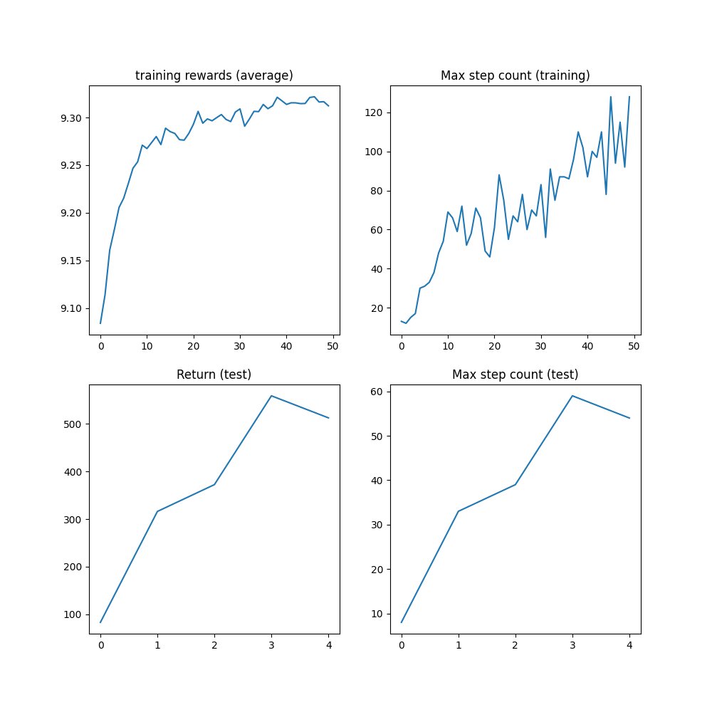
结果 ¶

在达到 1M 步数上限之前，算法的最大 步数应达到 1000 步，这是 轨迹被截断之前的最大步数。

plt.figure(figsize=(10, 10))
plt.subplot(2, 2, 1)
plt.plot(logs["reward"])
plt.title("training rewards (average)")
plt.subplot(2, 2, 2)
plt.plot(logs["step_count"])
plt.title("Max step count (training)")
plt.subplot(2, 2, 3)
plt.plot(logs["eval reward (sum)"])
plt.title("Return (test)")
plt.subplot(2, 2, 4)
plt.plot(logs["eval step_count"])
plt.title("Max step count (test)")
plt.show()

结论和后续步骤 ¶

在本教程中，我们学习了：

1. 如何使用 torchrl 创建和自定义环境 ; 2.如何编写模型和损失函数； 3.如何设置典型的训练循环。

如果您想进一步尝试本教程，可以应用以下修改：

• 从效率角度来看， 我们可以并行运行多个模拟以加快数据收集速度。 检查 ParallelEnv 了解更多信息。
• 从日志记录的角度来看，可以添加一个 torchrl.record.VideoRecorder 转换请求渲染后 到环境以获得正在运行的倒立摆的视觉渲染。检查 torchrl.record 了解更多信息。

脚本的总运行时间： (4 分 40.737 秒)

---

我们一直在努力

apachecn/AiLearning

---