PyTorch 的 TensorBoard 支持
译者:Fadegentle
项目地址:https://pytorch.apachecn.org/2.0/tutorials/beginner/introyt/tensorboardyt_tutorial
原始地址:https://pytorch.org/tutorials/beginner/introyt/tensorboardyt_tutorial.html
请跟随下面的视频或在 youtube 上观看。
开始之前
运行本教程前,需要安装 PyTorch、TorchVision、Matplotlib 和 TensorBoard。
使用 conda 安装:
使用 pip 安装:
安装依赖项后,在安装依赖项的 Python 环境中重启本笔记本。
入门
此笔记本中,我们将针对 Fashion-MNIST 数据集训练 LeNet-5 的一个变体。Fashion-MNIST 是一组描绘各种服装的图片,其中有十个类标签表示所描绘服装的类型。
# PyTorch model and training necessities
import torch
import torch.nn as nn
import torch.nn.functional as F
import torch.optim as optim

# Image datasets and image manipulation
import torchvision
import torchvision.transforms as transforms

# Image display
import matplotlib.pyplot as plt
import numpy as np

# PyTorch TensorBoard support
from torch.utils.tensorboard import SummaryWriter

# In case you are using an environment that has TensorFlow installed,
# such as Google Colab, uncomment the following code to avoid
# a bug with saving embeddings to your TensorBoard directory

# import tensorflow as tf
# import tensorboard as tb
# tf.io.gfile = tb.compat.tensorflow_stub.io.gfile
在 TensorBoard 中显示图像
让我们先将数据集中的样本图像添加到 TensorBoard:
# Gather datasets and prepare them for consumption
transform = transforms.Compose(
    [transforms.ToTensor(),
    transforms.Normalize((0.5,), (0.5,))])

# Store separate training and validations splits in ./data
training_set = torchvision.datasets.FashionMNIST('./data',
    download=True,
    train=True,
    transform=transform)
validation_set = torchvision.datasets.FashionMNIST('./data',
    download=True,
    train=False,
    transform=transform)

training_loader = torch.utils.data.DataLoader(training_set,
                                              batch_size=4,
                                              shuffle=True,
                                              num_workers=2)


validation_loader = torch.utils.data.DataLoader(validation_set,
                                                batch_size=4,
                                                shuffle=False,
                                                num_workers=2)

# Class labels
classes = ('T-shirt/top', 'Trouser', 'Pullover', 'Dress', 'Coat',
        'Sandal', 'Shirt', 'Sneaker', 'Bag', 'Ankle Boot')

# Helper function for inline image display
def matplotlib_imshow(img, one_channel=False):
    if one_channel:
        img = img.mean(dim=0)
    img = img / 2 + 0.5     # unnormalize
    npimg = img.numpy()
    if one_channel:
        plt.imshow(npimg, cmap="Greys")
    else:
        plt.imshow(np.transpose(npimg, (1, 2, 0)))

# Extract a batch of 4 images
dataiter = iter(training_loader)
images, labels = next(dataiter)

# Create a grid from the images and show them
img_grid = torchvision.utils.make_grid(images)
matplotlib_imshow(img_grid, one_channel=True)
Downloading http://fashion-mnist.s3-website.eu-central-1.amazonaws.com/train-images-idx3-ubyte.gz
Downloading http://fashion-mnist.s3-website.eu-central-1.amazonaws.com/train-images-idx3-ubyte.gz to ./data/FashionMNIST/raw/train-images-idx3-ubyte.gz

  0%|          | 0/26421880 [00:00<?, ?it/s]
  0%|          | 65536/26421880 [00:00<01:12, 365681.82it/s]
  1%|          | 229376/26421880 [00:00<00:38, 684388.67it/s]
  2%|2         | 589824/26421880 [00:00<00:16, 1595384.58it/s]
  6%|6         | 1638400/26421880 [00:00<00:06, 3604619.30it/s]
 12%|#2        | 3178496/26421880 [00:00<00:03, 6701731.95it/s]
 21%|##        | 5505024/26421880 [00:00<00:02, 9497525.59it/s]
 30%|##9       | 7831552/26421880 [00:01<00:01, 12814081.64it/s]
 39%|###8      | 10289152/26421880 [00:01<00:01, 13504284.18it/s]
 47%|####7     | 12484608/26421880 [00:01<00:00, 15405490.54it/s]
 57%|#####7    | 15073280/26421880 [00:01<00:00, 15405814.47it/s]
 65%|######4   | 17104896/26421880 [00:01<00:00, 16441216.54it/s]
 75%|#######5  | 19857408/26421880 [00:01<00:00, 16433922.86it/s]
 82%|########2 | 21757952/26421880 [00:01<00:00, 16880509.87it/s]
 93%|#########3| 24641536/26421880 [00:01<00:00, 16974431.24it/s]
100%|#########9| 26378240/26421880 [00:02<00:00, 16975657.90it/s]
100%|##########| 26421880/26421880 [00:02<00:00, 12640201.24it/s]
Extracting ./data/FashionMNIST/raw/train-images-idx3-ubyte.gz to ./data/FashionMNIST/raw

Downloading http://fashion-mnist.s3-website.eu-central-1.amazonaws.com/train-labels-idx1-ubyte.gz
Downloading http://fashion-mnist.s3-website.eu-central-1.amazonaws.com/train-labels-idx1-ubyte.gz to ./data/FashionMNIST/raw/train-labels-idx1-ubyte.gz

  0%|          | 0/29515 [00:00<?, ?it/s]
100%|##########| 29515/29515 [00:00<00:00, 328611.58it/s]
Extracting ./data/FashionMNIST/raw/train-labels-idx1-ubyte.gz to ./data/FashionMNIST/raw

Downloading http://fashion-mnist.s3-website.eu-central-1.amazonaws.com/t10k-images-idx3-ubyte.gz
Downloading http://fashion-mnist.s3-website.eu-central-1.amazonaws.com/t10k-images-idx3-ubyte.gz to ./data/FashionMNIST/raw/t10k-images-idx3-ubyte.gz

  0%|          | 0/4422102 [00:00<?, ?it/s]
  1%|1         | 65536/4422102 [00:00<00:12, 363006.91it/s]
  5%|5         | 229376/4422102 [00:00<00:06, 686330.69it/s]
 20%|##        | 884736/4422102 [00:00<00:01, 2499866.60it/s]
 44%|####3     | 1933312/4422102 [00:00<00:00, 4140114.20it/s]
100%|##########| 4422102/4422102 [00:00<00:00, 6109767.16it/s]
Extracting ./data/FashionMNIST/raw/t10k-images-idx3-ubyte.gz to ./data/FashionMNIST/raw

Downloading http://fashion-mnist.s3-website.eu-central-1.amazonaws.com/t10k-labels-idx1-ubyte.gz
Downloading http://fashion-mnist.s3-website.eu-central-1.amazonaws.com/t10k-labels-idx1-ubyte.gz to ./data/FashionMNIST/raw/t10k-labels-idx1-ubyte.gz

  0%|          | 0/5148 [00:00<?, ?it/s]
100%|##########| 5148/5148 [00:00<00:00, 39330194.89it/s]
Extracting ./data/FashionMNIST/raw/t10k-labels-idx1-ubyte.gz to ./data/FashionMNIST/raw
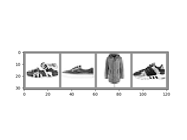
上面,我们使用 TorchVision 和 Matplotlib 为输入的小批量数据创建了一个可视化网格。下面,我们调用 SummaryWriter 的 add_image() 来记录图像供 TensorBoard 使用,同时还调用 flush() 确保图像立即写入磁盘。
# Default log_dir argument is "runs" - but it's good to be specific
# torch.utils.tensorboard.SummaryWriter is imported above
writer = SummaryWriter('runs/fashion_mnist_experiment_1')

# Write image data to TensorBoard log dir
writer.add_image('Four Fashion-MNIST Images', img_grid)
writer.flush()

# To view, start TensorBoard on the command line with:
#   tensorboard --logdir=runs
# ...and open a browser tab to http://localhost:6006/
如果在命令行下启动 TensorBoard 并在新的浏览器标签页中(一般是 localhost:6006)打开它,就能在“IMAGES”标签页下看到图像网格。
绘制标量图以可视化训练
TensorBoard 可用于跟踪训练的进度和效果。下面,我们将运行一个训练循环,跟踪一些指标,并保存数据供 TensorBoard 使用。
让我们定义一个模型来对图块进行分类,并定义一个优化器和损失函数来进行训练:
class Net(nn.Module):
    def __init__(self):
        super(Net, self).__init__()
        self.conv1 = nn.Conv2d(1, 6, 5)
        self.pool = nn.MaxPool2d(2, 2)
        self.conv2 = nn.Conv2d(6, 16, 5)
        self.fc1 = nn.Linear(16 * 4 * 4, 120)
        self.fc2 = nn.Linear(120, 84)
        self.fc3 = nn.Linear(84, 10)

    def forward(self, x):
        x = self.pool(F.relu(self.conv1(x)))
        x = self.pool(F.relu(self.conv2(x)))
        x = x.view(-1, 16 * 4 * 4)
        x = F.relu(self.fc1(x))
        x = F.relu(self.fc2(x))
        x = self.fc3(x)
        return x


net = Net()
criterion = nn.CrossEntropyLoss()
optimizer = optim.SGD(net.parameters(), lr=0.001, momentum=0.9)
现在,让我们训练一个周期,并每 1000 次评估一下训练集与验证集的损失:
print(len(validation_loader))
for epoch in range(1):  # loop over the dataset multiple times
    running_loss = 0.0

    for i, data in enumerate(training_loader, 0):
        # basic training loop
        inputs, labels = data
        optimizer.zero_grad()
        outputs = net(inputs)
        loss = criterion(outputs, labels)
        loss.backward()
        optimizer.step()

        running_loss += loss.item()
        if i % 1000 == 999:    # Every 1000 mini-batches...
            print('Batch {}'.format(i + 1))
            # Check against the validation set
            running_vloss = 0.0

            net.train(False) # Don't need to track gradents for validation
            for j, vdata in enumerate(validation_loader, 0):
                vinputs, vlabels = vdata
                voutputs = net(vinputs)
                vloss = criterion(voutputs, vlabels)
                running_vloss += vloss.item()
            net.train(True) # Turn gradients back on for training

            avg_loss = running_loss / 1000
            avg_vloss = running_vloss / len(validation_loader)

            # Log the running loss averaged per batch
            writer.add_scalars('Training vs. Validation Loss',
                            { 'Training' : avg_loss, 'Validation' : avg_vloss },
                            epoch * len(training_loader) + i)

            running_loss = 0.0
print('Finished Training')
writer.flush()
输出:
2500
Batch 1000
Batch 2000
Batch 3000
Batch 4000
Batch 5000
Batch 6000
Batch 7000
Batch 8000
Batch 9000
Batch 10000
Batch 11000
Batch 12000
Batch 13000
Batch 14000
Batch 15000
Finished Training
切换到打开的 TensorBoard,查看“SCALARS”标签页。
可视化模型
TensorBoard 还可用于检查模型内的数据流。为此,请使用模型和样本输入调用 add_graph() 方法。打开
# Again, grab a single mini-batch of images
dataiter = iter(training_loader)
images, labels = next(dataiter)

# add_graph() will trace the sample input through your model,
# and render it as a graph.
writer.add_graph(net, images)
writer.flush()
切换到 TensorBoard 时,您应该会看到“GRAPHS”标签页。双击“NET”节点,查看模型中的层和数据流。
使用嵌入可视化数据集
我们使用的 28 x 28 的图块可以建模为 784 维向量(28 * 28 = 784),将其投影到更低维度的表示中会很有帮助。add_embedding() 方法会将一组数据投影到方差最大的三个维度上,并自动以交互式 3D 图表的形式显示出来。
下面,我们将获取数据样本,并生成这样的嵌入:
# Select a random subset of data and corresponding labels
def select_n_random(data, labels, n=100):
    assert len(data) == len(labels)

    perm = torch.randperm(len(data))
    return data[perm][:n], labels[perm][:n]

# Extract a random subset of data
images, labels = select_n_random(training_set.data, training_set.targets)

# get the class labels for each image
class_labels = [classes[label] for label in labels]

# log embeddings
features = images.view(-1, 28 * 28)
writer.add_embedding(features,
                    metadata=class_labels,
                    label_img=images.unsqueeze(1))
writer.flush()
writer.close()
现在,如果切换到 TensorBoard 并选择“PROJECTOR”标签页,就会看到投影的 3D 呈现。你可以旋转和缩放模型。仔细观察不同尺度下的模型,看看是否能在投影数据和标签聚类中发现套路。
为获得更好的可视性,建议采用以下方法:
- 从左侧的“Color by”下拉菜单中选择“label”。
- 切换顶部的“Night Mode”图标,将浅色图像放在深色背景上。
其它资源
更多信息,请参阅:
- PyTorch 文档中的 torch.utils.tensorboard.SummaryWriter
- PyTorch.org 教程中的 TensorBoard 教程内容
- TensorBoard 文档中的更多信息
