使用 nn.Transformer 和 torchtext 进行语言建模 
项目地址:https://pytorch.apachecn.org/2.0/tutorials/beginner/transformer_tutorial
原始地址:https://pytorch.org/tutorials/beginner/transformer_tutorial.html
这是一个关于训练模型以使用 nn.Transformer 预测序列中下一个单词的教程模块。
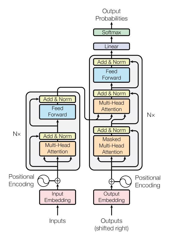
PyTorch 1.2 版本包含一个基于论文的标准转换器模块 Attention is All You Need.与循环神经网络相比 ( RNN)中,Transformer 模型已被证明对于许多序列到序列任务来说质量优越,同时具有更强的可并行性。 nn.Transformer 模块完全依赖于注意力机制(实现为 nn.MultiheadAttention )绘制输入和输出之间的全局依赖关系。 nn.Transformer 模块是高度模块化的,因此单个组件(例如, nn.TransformerEncoder )可以轻松改编/组合。
定义模型 
在本教程中,我们在因果语言建模任务上训练 nn.TransformerEncoder 模型。请注意,本教程不涵盖 nn.TransformerDecoder 的训练 ,如上图右半部分所示。语言建模任务是为给定单词(或单词序列)跟随单词序列的可能性分配概率。首先将标记序列传递到嵌入层,然后是位置编码层来解释单词的顺序(有关更多详细信息,请参阅下一段)。 nn.TransformerEncoder 由多个层组成 nn.TransformerEncoderLayer.
对于输入序列,需要一个方形注意掩码,因为“nn.TransformerDecoder”中的自注意层只允许出现序列中较早的位置。对于语言建模任务,未来位置上的任何标记都应该被屏蔽。这种掩蔽与输出嵌入与后面位置偏移的事实相结合,确保位置 i 的预测只能依赖于小于 i 的位置处的已知输出。为了生成输出词的概率分布,的输出 nn.TransformerEncoder 模型通过线性层来输出非归一化 logits。由于稍后使用了 CrossEntropyLoss ,这要求输入是非标准化的 logits。
import math
import os
from tempfile import TemporaryDirectory
from typing import Tuple

import torch
from torch import nn, Tensor
from torch.nn import TransformerEncoder, TransformerEncoderLayer
from torch.utils.data import dataset

class TransformerModel(nn.Module):

    def __init__(self, ntoken: int, d_model: int, nhead: int, d_hid: int,
                 nlayers: int, dropout: float = 0.5):
        super().__init__()
        self.model_type = 'Transformer'
        self.pos_encoder = PositionalEncoding(d_model, dropout)
        encoder_layers = TransformerEncoderLayer(d_model, nhead, d_hid, dropout)
        self.transformer_encoder = TransformerEncoder(encoder_layers, nlayers)
        self.embedding = nn.Embedding(ntoken, d_model)
        self.d_model = d_model
        self.linear = nn.Linear(d_model, ntoken)

        self.init_weights()

    def init_weights(self) -> None:
        initrange = 0.1
        self.embedding.weight.data.uniform_(-initrange, initrange)
        self.linear.bias.data.zero_()
        self.linear.weight.data.uniform_(-initrange, initrange)

    def forward(self, src: Tensor, src_mask: Tensor = None) -> Tensor:
 """
 Arguments:
 src: Tensor, shape ``[seq_len, batch_size]``
 src_mask: Tensor, shape ``[seq_len, seq_len]``

 Returns:
 output Tensor of shape ``[seq_len, batch_size, ntoken]``
 """
        src = self.embedding(src) * math.sqrt(self.d_model)
        src = self.pos_encoder(src)
        if src_mask is None:
 """Generate a square causal mask for the sequence. The masked positions are filled with float('-inf').
 Unmasked positions are filled with float(0.0).
 """
            src_mask = nn.Transformer.generate_square_subsequent_mask(len(src)).to(device)
        output = self.transformer_encoder(src, src_mask)
        output = self.linear(output)
        return output
PositionalEncoding 模块注入一些有关序列中标记的相对或绝对位置的信息。位置编码与嵌入具有相同的维度,因此可以将两者相加。在这里,我们使用不同频率的 sine 和 cosine 函数。
class PositionalEncoding(nn.Module):

    def __init__(self, d_model: int, dropout: float = 0.1, max_len: int = 5000):
        super().__init__()
        self.dropout = nn.Dropout(p=dropout)

        position = torch.arange(max_len).unsqueeze(1)
        div_term = torch.exp(torch.arange(0, d_model, 2) * (-math.log(10000.0) / d_model))
        pe = torch.zeros(max_len, 1, d_model)
        pe[:, 0, 0::2] = torch.sin(position * div_term)
        pe[:, 0, 1::2] = torch.cos(position * div_term)
        self.register_buffer('pe', pe)

    def forward(self, x: Tensor) -> Tensor:
 """
 Arguments:
 x: Tensor, shape ``[seq_len, batch_size, embedding_dim]``
 """
        x = x + self.pe[:x.size(0)]
        return self.dropout(x)
加载并批处理数据 
本教程使用 torchtext 生成 Wikitext-2 数据集。要访问 torchtext 数据集,请按照以下位置的说明安装 torchdata https://github.com/pytorch/data 。
vocab 对象是基于训练数据集构建的,用于将 token 数值化为tensor。 Wikitext-2 代表 rare tokens <unk>
给定一个连续数据的一维向量, batchify() 将数据 排列到 batch_size 列。如果数据没有均匀地分为 batch_size 列,则数据将被修剪以适合。例如,以字母表作为数据(总长度为 26)和 batch_size=4,我们将将字母表划分为长度为 6 的序列,从而得到 4 个这样的序列.
批处理可实现更多并行处理。然而,批处理意味着模型独立处理每一列;例如,在上面的示例中无法学习 G 和 F 的依赖关系。
from torchtext.datasets import WikiText2
from torchtext.data.utils import get_tokenizer
from torchtext.vocab import build_vocab_from_iterator

train_iter = WikiText2(split='train')
tokenizer = get_tokenizer('basic_english')
vocab = build_vocab_from_iterator(map(tokenizer, train_iter), specials=['<unk>'])
vocab.set_default_index(vocab['<unk>'])

def data_process(raw_text_iter: dataset.IterableDataset) -> Tensor:
 """Converts raw text into a flat Tensor."""
    data = [torch.tensor(vocab(tokenizer(item)), dtype=torch.long) for item in raw_text_iter]
    return torch.cat(tuple(filter(lambda t: t.numel() > 0, data)))

# ``train_iter`` was "consumed" by the process of building the vocab,
# so we have to create it again
train_iter, val_iter, test_iter = WikiText2()
train_data = data_process(train_iter)
val_data = data_process(val_iter)
test_data = data_process(test_iter)

device = torch.device('cuda' if torch.cuda.is_available() else 'cpu')

def batchify(data: Tensor, bsz: int) -> Tensor:
 """Divides the data into ``bsz`` separate sequences, removing extra elements
 that wouldn't cleanly fit.

 Arguments:
 data: Tensor, shape ``[N]``
 bsz: int, batch size

 Returns:
 Tensor of shape ``[N // bsz, bsz]``
 """
    seq_len = data.size(0) // bsz
    data = data[:seq_len * bsz]
    data = data.view(bsz, seq_len).t().contiguous()
    return data.to(device)

batch_size = 20
eval_batch_size = 10
train_data = batchify(train_data, batch_size)  # shape ``[seq_len, batch_size]``
val_data = batchify(val_data, eval_batch_size)
test_data = batchify(test_data, eval_batch_size)
生成输入和目标序列的函数 
get_batch() 为变压器模型生成一对输入目标序列。它将源数据细分为length bptt 的块。对于语言建模任务,模型需要以下单词作为 Target 。例如, bptt 值为 2,we’d 会为 i = 0 获取以下两个变量:
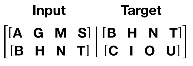
需要注意的是,块沿着维度 0,与中的 S 维度一致变压器模型。批次维度 N 沿维度 1。
bptt = 35
def get_batch(source: Tensor, i: int) -> Tuple[Tensor, Tensor]:
 """
 Args:
 source: Tensor, shape ``[full_seq_len, batch_size]``
 i: int

 Returns:
 tuple (data, target), where data has shape ``[seq_len, batch_size]`` and
 target has shape ``[seq_len * batch_size]``
 """
    seq_len = min(bptt, len(source) - 1 - i)
    data = source[i:i+seq_len]
    target = source[i+1:i+1+seq_len].reshape(-1)
    return data, target
启动实例 
模型超参数定义如下。 vocab 大小等于 vocab 对象的长度。
ntokens = len(vocab)  # size of vocabulary
emsize = 200  # embedding dimension
d_hid = 200  # dimension of the feedforward network model in ``nn.TransformerEncoder``
nlayers = 2  # number of ``nn.TransformerEncoderLayer`` in ``nn.TransformerEncoder``
nhead = 2  # number of heads in ``nn.MultiheadAttention``
dropout = 0.2  # dropout probability
model = TransformerModel(ntokens, emsize, nhead, d_hid, nlayers, dropout).to(device)
输出:
/opt/conda/envs/py_3.10/lib/python3.10/site-packages/torch/nn/modules/transformer.py:282: UserWarning:

enable_nested_tensor is True, but self.use_nested_tensor is False because encoder_layer.self_attn.batch_first was not True(use batch_first for better inference performance)
运行模型 
我们使用 CrossEntropyLoss 和 SGD (随机梯度下降)优化器。学习率最初设置为5.0,并遵循 StepLR 时间表。在训练过程中,我们使用 nn.utils.clip_grad_norm_以防止梯度爆炸。
import time

criterion = nn.CrossEntropyLoss()
lr = 5.0  # learning rate
optimizer = torch.optim.SGD(model.parameters(), lr=lr)
scheduler = torch.optim.lr_scheduler.StepLR(optimizer, 1.0, gamma=0.95)

def train(model: nn.Module) -> None:
    model.train()  # turn on train mode
    total_loss = 0.
    log_interval = 200
    start_time = time.time()

    num_batches = len(train_data) // bptt
    for batch, i in enumerate(range(0, train_data.size(0) - 1, bptt)):
        data, targets = get_batch(train_data, i)
        output = model(data)
        output_flat = output.view(-1, ntokens)
        loss = criterion(output_flat, targets)

        optimizer.zero_grad()
        loss.backward()
        torch.nn.utils.clip_grad_norm_(model.parameters(), 0.5)
        optimizer.step()

        total_loss += loss.item()
        if batch % log_interval == 0 and batch > 0:
            lr = scheduler.get_last_lr()[0]
            ms_per_batch = (time.time() - start_time) * 1000 / log_interval
            cur_loss = total_loss / log_interval
            ppl = math.exp(cur_loss)
            print(f'| epoch {epoch:3d} | {batch:5d}/{num_batches:5d} batches | '
                  f'lr {lr:02.2f} | ms/batch {ms_per_batch:5.2f} | '
                  f'loss {cur_loss:5.2f} | ppl {ppl:8.2f}')
            total_loss = 0
            start_time = time.time()

def evaluate(model: nn.Module, eval_data: Tensor) -> float:
    model.eval()  # turn on evaluation mode
    total_loss = 0.
    with torch.no_grad():
        for i in range(0, eval_data.size(0) - 1, bptt):
            data, targets = get_batch(eval_data, i)
            seq_len = data.size(0)
            output = model(data)
            output_flat = output.view(-1, ntokens)
            total_loss += seq_len * criterion(output_flat, targets).item()
    return total_loss / (len(eval_data) - 1)
循环纪元。如果验证损失是迄今为止我们’见过的最好的,则保存模型。在每个时期后调整学习率。
best_val_loss = float('inf')
epochs = 3

with TemporaryDirectory() as tempdir:
    best_model_params_path = os.path.join(tempdir, "best_model_params.pt")

    for epoch in range(1, epochs + 1):
        epoch_start_time = time.time()
        train(model)
        val_loss = evaluate(model, val_data)
        val_ppl = math.exp(val_loss)
        elapsed = time.time() - epoch_start_time
        print('-' * 89)
        print(f'| end of epoch {epoch:3d} | time: {elapsed:5.2f}s | '
            f'valid loss {val_loss:5.2f} | valid ppl {val_ppl:8.2f}')
        print('-' * 89)

        if val_loss < best_val_loss:
            best_val_loss = val_loss
            torch.save(model.state_dict(), best_model_params_path)

        scheduler.step()
    model.load_state_dict(torch.load(best_model_params_path)) # load best model states
输出:
| epoch   1 |   200/ 2928 batches | lr 5.00 | ms/batch 31.82 | loss  8.19 | ppl  3613.91
| epoch   1 |   400/ 2928 batches | lr 5.00 | ms/batch 28.69 | loss  6.88 | ppl   970.94
| epoch   1 |   600/ 2928 batches | lr 5.00 | ms/batch 28.53 | loss  6.43 | ppl   621.40
| epoch   1 |   800/ 2928 batches | lr 5.00 | ms/batch 28.66 | loss  6.30 | ppl   542.89
| epoch   1 |  1000/ 2928 batches | lr 5.00 | ms/batch 28.34 | loss  6.18 | ppl   484.73
| epoch   1 |  1200/ 2928 batches | lr 5.00 | ms/batch 28.26 | loss  6.15 | ppl   467.52
| epoch   1 |  1400/ 2928 batches | lr 5.00 | ms/batch 28.41 | loss  6.11 | ppl   450.65
| epoch   1 |  1600/ 2928 batches | lr 5.00 | ms/batch 28.31 | loss  6.11 | ppl   450.73
| epoch   1 |  1800/ 2928 batches | lr 5.00 | ms/batch 28.22 | loss  6.02 | ppl   410.39
| epoch   1 |  2000/ 2928 batches | lr 5.00 | ms/batch 28.41 | loss  6.01 | ppl   409.43
| epoch   1 |  2200/ 2928 batches | lr 5.00 | ms/batch 28.30 | loss  5.89 | ppl   361.18
| epoch   1 |  2400/ 2928 batches | lr 5.00 | ms/batch 28.23 | loss  5.97 | ppl   393.23
| epoch   1 |  2600/ 2928 batches | lr 5.00 | ms/batch 28.42 | loss  5.95 | ppl   383.85
| epoch   1 |  2800/ 2928 batches | lr 5.00 | ms/batch 28.27 | loss  5.88 | ppl   357.86
-----------------------------------------------------------------------------------------
| end of epoch   1 | time: 86.83s | valid loss  5.78 | valid ppl   324.74
-----------------------------------------------------------------------------------------
| epoch   2 |   200/ 2928 batches | lr 4.75 | ms/batch 28.52 | loss  5.86 | ppl   349.96
| epoch   2 |   400/ 2928 batches | lr 4.75 | ms/batch 28.33 | loss  5.85 | ppl   348.22
| epoch   2 |   600/ 2928 batches | lr 4.75 | ms/batch 28.25 | loss  5.66 | ppl   286.86
| epoch   2 |   800/ 2928 batches | lr 4.75 | ms/batch 28.41 | loss  5.70 | ppl   297.60
| epoch   2 |  1000/ 2928 batches | lr 4.75 | ms/batch 28.34 | loss  5.64 | ppl   282.01
| epoch   2 |  1200/ 2928 batches | lr 4.75 | ms/batch 28.31 | loss  5.67 | ppl   290.49
| epoch   2 |  1400/ 2928 batches | lr 4.75 | ms/batch 28.38 | loss  5.68 | ppl   292.36
| epoch   2 |  1600/ 2928 batches | lr 4.75 | ms/batch 28.32 | loss  5.70 | ppl   299.93
| epoch   2 |  1800/ 2928 batches | lr 4.75 | ms/batch 28.30 | loss  5.64 | ppl   282.54
| epoch   2 |  2000/ 2928 batches | lr 4.75 | ms/batch 28.41 | loss  5.66 | ppl   288.23
| epoch   2 |  2200/ 2928 batches | lr 4.75 | ms/batch 28.34 | loss  5.54 | ppl   254.44
| epoch   2 |  2400/ 2928 batches | lr 4.75 | ms/batch 28.30 | loss  5.65 | ppl   282.92
| epoch   2 |  2600/ 2928 batches | lr 4.75 | ms/batch 28.45 | loss  5.64 | ppl   282.54
| epoch   2 |  2800/ 2928 batches | lr 4.75 | ms/batch 28.32 | loss  5.58 | ppl   263.76
-----------------------------------------------------------------------------------------
| end of epoch   2 | time: 86.04s | valid loss  5.65 | valid ppl   282.95
-----------------------------------------------------------------------------------------
| epoch   3 |   200/ 2928 batches | lr 4.51 | ms/batch 28.66 | loss  5.60 | ppl   270.97
| epoch   3 |   400/ 2928 batches | lr 4.51 | ms/batch 28.40 | loss  5.62 | ppl   276.79
| epoch   3 |   600/ 2928 batches | lr 4.51 | ms/batch 28.33 | loss  5.42 | ppl   226.33
| epoch   3 |   800/ 2928 batches | lr 4.51 | ms/batch 28.42 | loss  5.48 | ppl   239.30
| epoch   3 |  1000/ 2928 batches | lr 4.51 | ms/batch 28.32 | loss  5.44 | ppl   229.71
| epoch   3 |  1200/ 2928 batches | lr 4.51 | ms/batch 28.32 | loss  5.48 | ppl   238.78
| epoch   3 |  1400/ 2928 batches | lr 4.51 | ms/batch 28.39 | loss  5.50 | ppl   243.54
| epoch   3 |  1600/ 2928 batches | lr 4.51 | ms/batch 28.31 | loss  5.52 | ppl   248.47
| epoch   3 |  1800/ 2928 batches | lr 4.51 | ms/batch 28.35 | loss  5.46 | ppl   235.26
| epoch   3 |  2000/ 2928 batches | lr 4.51 | ms/batch 28.39 | loss  5.48 | ppl   240.24
| epoch   3 |  2200/ 2928 batches | lr 4.51 | ms/batch 28.36 | loss  5.38 | ppl   217.29
| epoch   3 |  2400/ 2928 batches | lr 4.51 | ms/batch 28.33 | loss  5.47 | ppl   236.64
| epoch   3 |  2600/ 2928 batches | lr 4.51 | ms/batch 28.37 | loss  5.47 | ppl   237.76
| epoch   3 |  2800/ 2928 batches | lr 4.51 | ms/batch 28.34 | loss  5.40 | ppl   220.67
-----------------------------------------------------------------------------------------
| end of epoch   3 | time: 86.11s | valid loss  5.61 | valid ppl   273.90
-----------------------------------------------------------------------------------------
评估测试数据集上的最佳模型 
test_loss = evaluate(model, test_data)
test_ppl = math.exp(test_loss)
print('=' * 89)
print(f'| End of training | test loss {test_loss:5.2f} | '
      f'test ppl {test_ppl:8.2f}')
print('=' * 89)
输出:
===================================================================================

| End of training | test loss  5.52 | test ppl   249.27
===================================================================================
脚本总运行时间: ( 4 分 29.085 秒)
